Getting Information on the peaks
We want to get the peaks from the spectra. We start importing and creating the TOF object with all isotopes from Ar and Kr
from tofsim import ToF
T = ToF('Ar,Kr')
T.Vs = 120                      # Extraction voltaje
T.Vd = 3000                     # Acceleration voltaje
T.signal();                     # Make the spectra
p = T.get_statistics_peaks() # Get the peaks
Here p is a dictionary-like object, where each key is a substance
and each value is a dictionary containing the information on the corresponding peak
p.keys()
dict_keys(['36Ar^{+}', '38Ar^{+}', '40Ar^{+}', '78Kr^{+}', '80Kr^{+}', '82Kr^{+}', '83Kr^{+}', '84Kr^{+}', '86Kr^{+}'])
list(p.values())[0]
{'index': (53, 56, 60),
 'position': 8.519009871520703,
 'height': 6.774956591427326,
 'width': 0.03684000090535555}
p.headers
['index', 'position', 'height', 'width']
Output the data of the peaks
print(p)
Substance    index              position      height      width
-----------  ---------------  ----------  ----------  ---------
36Ar^{+}     (53, 56, 60)        8.51901     6.77496  0.03684
38Ar^{+}     (97, 101, 104)      8.75419     1.28081  0.03684
40Ar^{+}     (140, 144, 147)     8.98108  2010.2      0.03684
78Kr^{+}     (816, 820, 825)    12.5402      6.76633  0.0473657
80Kr^{+}     (846, 851, 855)    12.7016     43.8943   0.0473657
82Kr^{+}     (876, 881, 885)    12.8594    222.046    0.0473657
83Kr^{+}     (891, 896, 900)    12.938     220.033    0.0473657
84Kr^{+}     (906, 910, 915)    13.0137   1079.69     0.0473657
86Kr^{+}     (935, 940, 944)    13.1696    329.294    0.0473657
If we want to print them in a different way we may use directly the
dictionary-like object or the list obtained by using tolist() method
pl = p.tolist()
pl[0]
['36Ar^{+}',
 (53, 56, 60),
 8.519009871520703,
 6.774956591427326,
 0.03684000090535555]
Importing and using the tabulate package we may output it to any supported format. For instance, “fancy_grid”:
from tabulate import tabulate
headers = ['Fragment'] + p.headers
print(tabulate(p.tolist(), headers=headers, tablefmt='fancy_grid'))
╒════════════╤═════════════════╤════════════╤════════════╤═══════════╕
│ Fragment   │ index           │   position │     height │     width │
╞════════════╪═════════════════╪════════════╪════════════╪═══════════╡
│ 36Ar^{+}   │ (53, 56, 60)    │    8.51901 │    6.77496 │ 0.03684   │
├────────────┼─────────────────┼────────────┼────────────┼───────────┤
│ 38Ar^{+}   │ (97, 101, 104)  │    8.75419 │    1.28081 │ 0.03684   │
├────────────┼─────────────────┼────────────┼────────────┼───────────┤
│ 40Ar^{+}   │ (140, 144, 147) │    8.98108 │ 2010.2     │ 0.03684   │
├────────────┼─────────────────┼────────────┼────────────┼───────────┤
│ 78Kr^{+}   │ (816, 820, 825) │   12.5402  │    6.76633 │ 0.0473657 │
├────────────┼─────────────────┼────────────┼────────────┼───────────┤
│ 80Kr^{+}   │ (846, 851, 855) │   12.7016  │   43.8943  │ 0.0473657 │
├────────────┼─────────────────┼────────────┼────────────┼───────────┤
│ 82Kr^{+}   │ (876, 881, 885) │   12.8594  │  222.046   │ 0.0473657 │
├────────────┼─────────────────┼────────────┼────────────┼───────────┤
│ 83Kr^{+}   │ (891, 896, 900) │   12.938   │  220.033   │ 0.0473657 │
├────────────┼─────────────────┼────────────┼────────────┼───────────┤
│ 84Kr^{+}   │ (906, 910, 915) │   13.0137  │ 1079.69    │ 0.0473657 │
├────────────┼─────────────────┼────────────┼────────────┼───────────┤
│ 86Kr^{+}   │ (935, 940, 944) │   13.1696  │  329.294   │ 0.0473657 │
╘════════════╧═════════════════╧════════════╧════════════╧═══════════╛
or “latex”:
print(tabulate(p.tolist(), headers=headers, tablefmt='latex'))
begin{tabular}{llrrr}
hline
 Fragment   & index           &   position &     height &     width \
hline
 36Ar^{}{+}   & (53, 56, 60)    &    8.51901 &    6.77496 & 0.03684   \
 38Ar^{}{+}   & (97, 101, 104)  &    8.75419 &    1.28081 & 0.03684   \
 40Ar^{}{+}   & (140, 144, 147) &    8.98108 & 2010.2     & 0.03684   \
 78Kr^{}{+}   & (816, 820, 825) &   12.5402  &    6.76633 & 0.0473657 \
 80Kr^{}{+}   & (846, 851, 855) &   12.7016  &   43.8943  & 0.0473657 \
 82Kr^{}{+}   & (876, 881, 885) &   12.8594  &  222.046   & 0.0473657 \
 83Kr^{}{+}   & (891, 896, 900) &   12.938   &  220.033   & 0.0473657 \
 84Kr^{}{+}   & (906, 910, 915) &   13.0137  & 1079.69    & 0.0473657 \
 86Kr^{}{+}   & (935, 940, 944) &   13.1696  &  329.294   & 0.0473657 \
hline
end{tabular}
Plot the data
import numpy as np
import matplotlib.pyplot as plt
pa = np.asarray(pl)
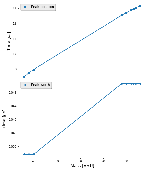
We will plot the position and width of each peak as a function of the mass of the fragment:
x = [T.fragments[k]['M'] for k in pa[:,0]]
ypos = pa[:,2]
ywidth = pa[:,4]
fig, ax = plt.subplots(nrows=2, sharex=True, figsize=(8, 10))
ax[0].plot(x, ypos, '-s', label='Peak position')
ax[1].plot(x, ywidth, '-o', label='Peak width')
ax[1].set_xlabel(r'Mass [AMU]')

ax[0].set_ylabel(r'Time [$\mu s$]')
ax[1].set_ylabel(r'Time [$\mu s$]')
ax[0].legend(loc='best')
ax[1].legend(loc='best')
plt.subplots_adjust(hspace=0)